Streamlit Guide
This guide covers the web-based interface of RegressionLab built with Streamlit. The Streamlit version provides a modern, browser-based experience for curve fitting operations.
Overview
The Streamlit interface offers:
Modern UI: Clean, intuitive design.
Accessibility: Works on any device with a browser.
No installation: Use the online version instantly.
Visual feedback: Real-time updates and progress indicators.
Easy sharing: Share results by downloading plots.
Configuration (language, UI colors, fonts, plot style, paths, etc.) is the same as the Tkinter app: edit the .env file or use the Tkinter Configure menu. The Streamlit UI has no in-app configuration dialog; it reads LANGUAGE, UI_BACKGROUND, UI_FOREGROUND, UI_BUTTON_*, UI_FONT_*, and the rest of the env schema. The initial language and the entire look (background, sidebar, buttons, text) follow the same rules as the desktop version. The sidebar is rendered slightly lighter than the main area for visual separation.
Accessing Streamlit
Online Version (Recommended)
Visit: https://regressionlab.streamlit.app/
First-time access:
Open the URL in your browser.
If you see “App is sleeping”, click “Start”.
Wait 30-60 seconds for the app to wake up.
The app will load and be ready to use.
Local Version
If you have RegressionLab installed locally:
Windows:
bin\run_streamlit.bat
macOS/Linux:
./bin/run_streamlit.sh
Or use the direct command:
streamlit run src/streamlit_app/app.py
The app will open automatically in your default browser at http://localhost:8501.
Interface Layout
The Streamlit interface consists of three main areas:
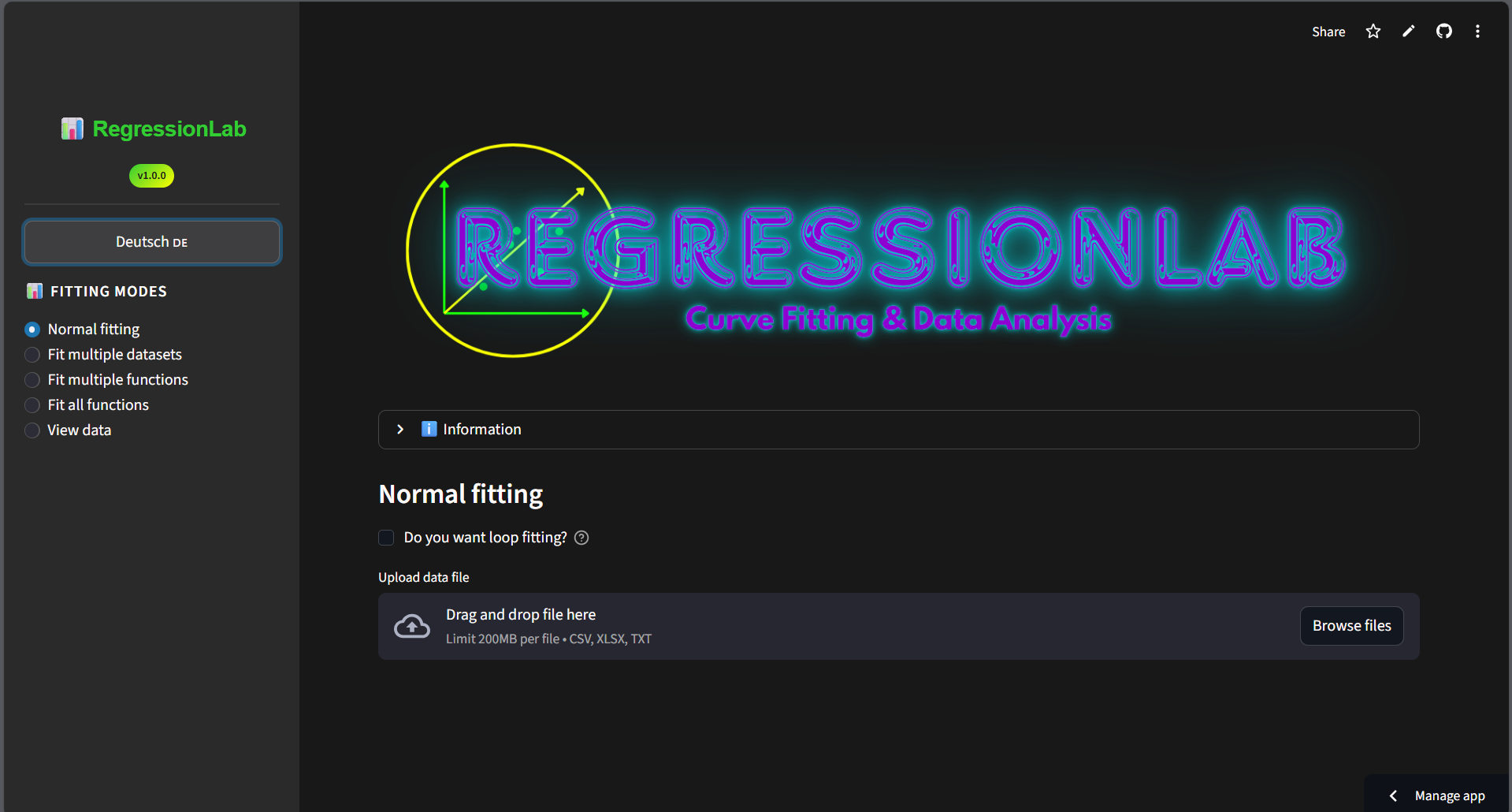
2. Main Area (Center)
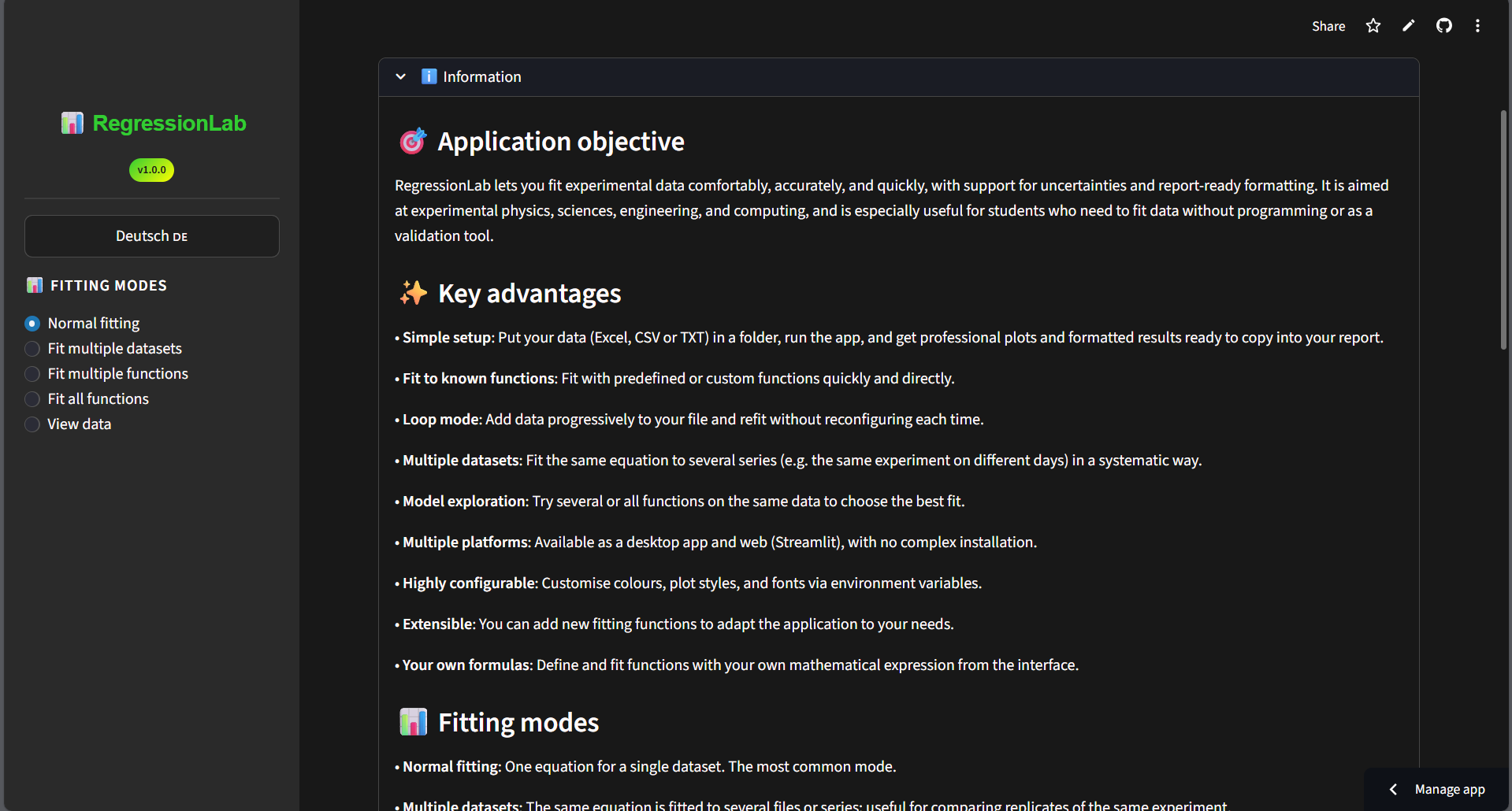
Logo and Title: RegressionLab branding.
Help Section: Expandable information about the app.
Operation Controls: File upload, variable selection, equation selection.
Results Display: Plots and fitting results.
3. Results Section (Bottom)
Three columns: Equation (formula and formatted equation, left), Parameters (fit parameters with uncertainties and IC 95%, center), Statistics (R², RMSE, χ², etc., right).
Plot Display: Visualization of fitted curves below the columns.
Download Button: Below each plot; save as PNG, JPG, or PDF (when configured).
Language Selection
Changing the Language
Look at the sidebar (left side).
Click the language button. The button always shows the next language in the cycle:
“English 🇬🇧” → switch to English (when current is Spanish).
“Deutsch 🇩🇪” → switch to German (when current is English).
“Español 🇪🇸” → switch to Spanish (when current is German).
The entire interface updates immediately. Click again to cycle to the next language.
Available Languages (cycle order: es → en → de → es):
Spanish (Español) – default.
English.
German (Deutsch).
Operation Modes
Mode 1: Normal Fitting
Purpose: Fit one equation to one dataset.
Steps:
Select Mode:
In the sidebar, ensure “Normal Fitting” is selected.
Optional: Loop fitting:
Check “Do you want loop fitting?” if you plan to fit another file with the same equation later.
When enabled, after the first fit an expander lets you upload another file and click “Fit again” without changing the equation.
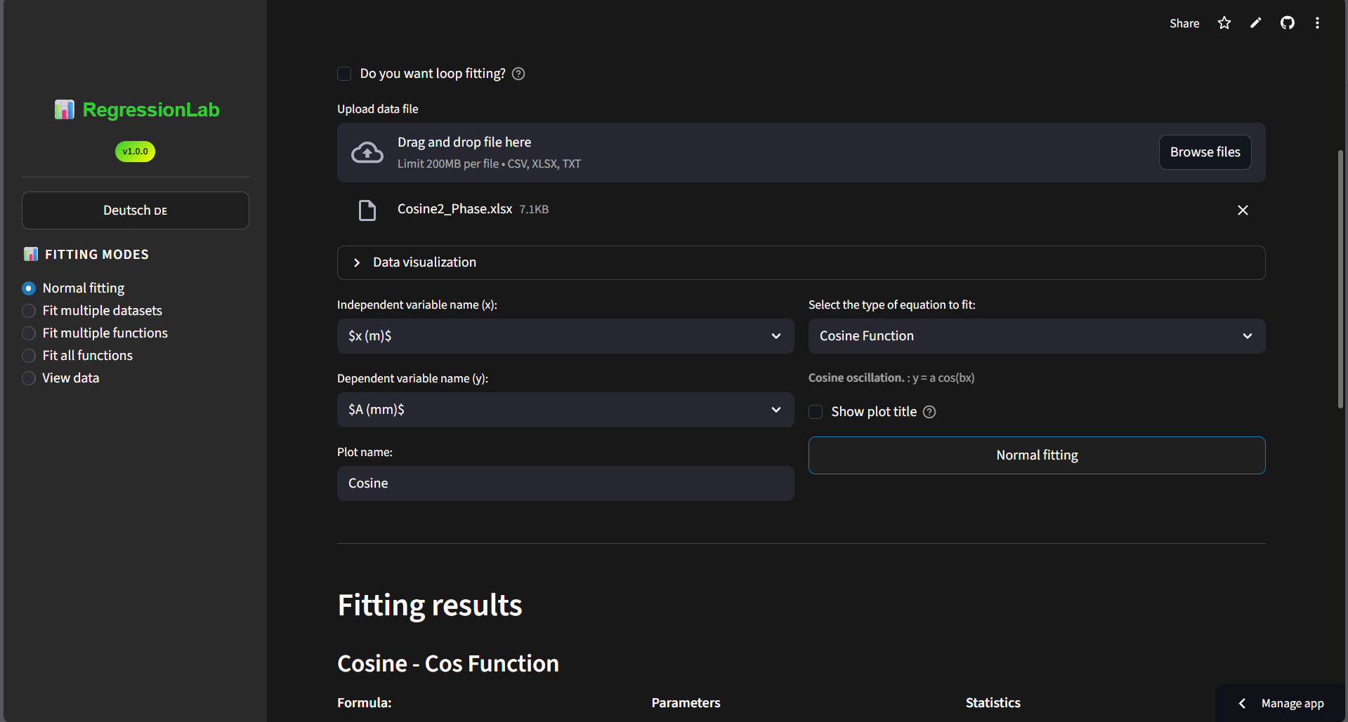
Upload Data:
Click “Browse files” or drag and drop your file.
Supported formats: CSV, XLSX, TXT.
Wait for the file to upload and process.
View Data (Optional):
Expand “Show Data” to preview your dataset.
Verify columns are loaded correctly.
Select Variables:
Independent Variable (X): Choose from dropdown (e.g., “time”).
Dependent Variable (Y): Choose from dropdown (e.g., “temperature”).
Plot Name: Enter a name for the output file (e.g., “experiment1”).
Select Equation:
Choose an equation type from the dropdown.
Options include Linear, Quadratic, Sine, Cosine, Logarithmic, etc.
Formula shown next to each option (e.g., “Linear with intercept - y=mx+n”).
Plot Options (optional):
Show plot title: Checkbox to show or hide the title on the plot. Default comes from the
PLOT_SHOW_TITLEenvironment variable; you can override it per fit without changing the config.
Fit the Curve:
Click “Normal Fitting” button (blue button).
Wait for processing (spinner appears).
Results appear below.
Review Results (three columns + plot):
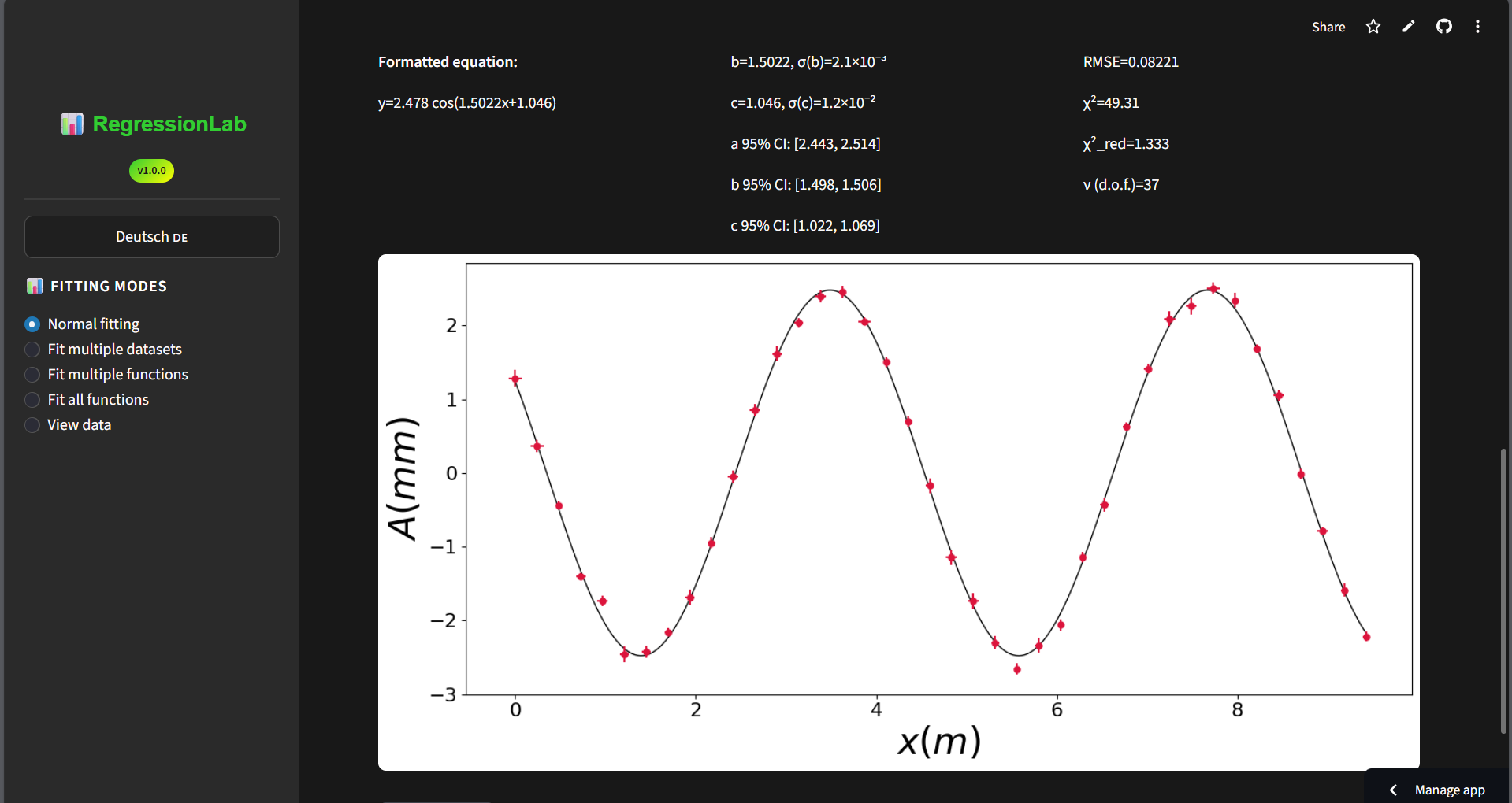
Equation (left): Formula and formatted equation with fitted values.
Parameters (center): Fit parameters (e.g. a, b, c) with uncertainties and IC 95%.
Statistics (right): R², RMSE, χ², χ²_red, degrees of freedom.
Plot: Data points and fitted curve below the columns (title uses the plot name if enabled).
Download: Button below the plot (PNG/JPG/PDF depending on configuration).
Download Plot:
Click the “📥 Download” button below the plot.
File format is that configured for the app (default PNG); if PDF is configured, the in-app preview is PNG but the download is PDF. The plot title (when shown) uses the plot name you entered; no numeric suffix is added.
Custom Formula:
If “Custom Formula” is selected:
Enter Number of Parameters: Use the number input (1-10).
Name Parameters: Enter names in the input boxes (e.g., “a”, “b”, “c”).
Enter Formula: Type your formula using Python syntax.
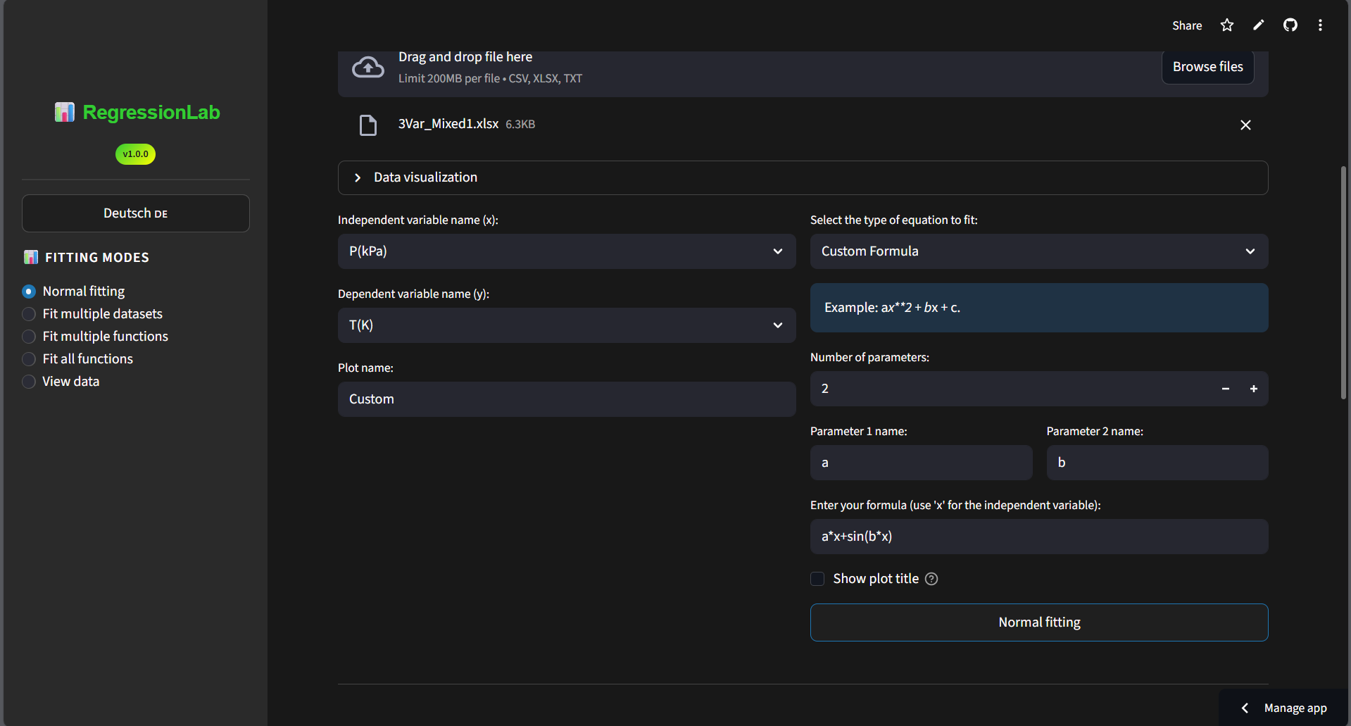
Example:
a*x**2 + b*x + c.Use
xas the independent variable.Use parameter names defined above.
Supported:
+,-,*,/,**(power),np.sin(),np.cos(),np.exp(),np.log(), etc.
Example Workflow:
1. Upload: temperature_experiment.csv
2. Select X: time, Y: temperature
3. Plot name: "temp_vs_time"
4. Equation: "Linear with intercept"
5. Click "Normal Fitting"
6. View results: y = 2.5·time + 20.3, R² = 0.98
7. Download plot
Mode 2: Multiple Datasets
Purpose: Apply the same equation to multiple different files.
Steps:
Select Mode:
In sidebar, click “Multiple Datasets”.
Select Equation First:
Choose the equation type you’ll use for all datasets.
If using custom formula, define it here.
Upload Multiple Files:
Click “Browse files”.
Hold Ctrl (Windows/Linux) or Cmd (Mac) to select multiple files.
Or use drag-and-drop for multiple files.
All files upload simultaneously.
Configure Each Dataset:
For each uploaded file:
File name shown as heading.
Select X variable.
Select Y variable.
Enter plot name (defaults to filename).
Plot Options (optional):
Show plot title: Checkbox to show or hide the title on all plots. Default from
PLOT_SHOW_TITLEenv var.
Fit All Datasets:
Click the “Multiple Datasets” button (centered, blue).
All datasets are fitted sequentially.
Progress indicators shown.
Review All Results:
Results displayed for each dataset.
Each has its own:
Equation.
Parameters.
Plot.
Download button.
Scroll through results to compare.
Tips:
All files should have similar column names.
X and Y variables can be different for each file if needed.
Results appear in upload order.
You can upload another set of files and click the button again for another round of fits with the same equation.
Example Workflow:
1. Equation: "Quadratic"
2. Upload 3 files:
   - sample1.csv
   - sample2.csv
   - sample3.csv
3. For each:
   - X: concentration
   - Y: absorbance
4. Click "Multiple Datasets"
5. Review 3 separate fit results
6. Compare parameters and R² values
Mode 3: Checker Fitting
Purpose: Test multiple equations on the same dataset to find the best fit.
Steps:
Select Mode:
In sidebar, click “Checker Fitting”.
Upload Data:
Upload your single data file.
Select Variables:
Choose X and Y variables.
Enter plot name.
Select Multiple Equations:
Click in the “Select equation” dropdown.
Select multiple options by clicking each one.
Options remain in the dropdown (multi-select).
Default: First 3 equations pre-selected.
Custom formulas not available in this mode.
Plot Options (optional):
Show plot title: Checkbox to show or hide the title on all plots. Default from
PLOT_SHOW_TITLEenv var.
Run Checker Fitting:
Click “Checker Fitting” button.
Progress bar shows completion.
Each equation fitted sequentially.
Compare Results:
All results displayed vertically.
Compare:
R² values (higher is better).
Visual fit quality in plots.
Parameter values.
Identify the best-fitting equation.
Example Workflow:
1. Upload: unknown_relationship.xlsx
2. X: voltage, Y: current
3. Select equations:
   - Linear with intercept (y=mx+n)
   - Quadratic (y=ax²)
   - Inverse (y=a/x)
   - Logarithmic (y=a·ln(x))
4. Click "Checker Fitting"
5. Compare results:
   - Linear: R²=0.75 (poor)
   - Quadratic: R²=0.92 (good)
   - Inverse: R²=0.98 (excellent!) ← Best fit
   - Logarithmic: R²=0.85 (acceptable)
6. Conclusion: Use inverse function
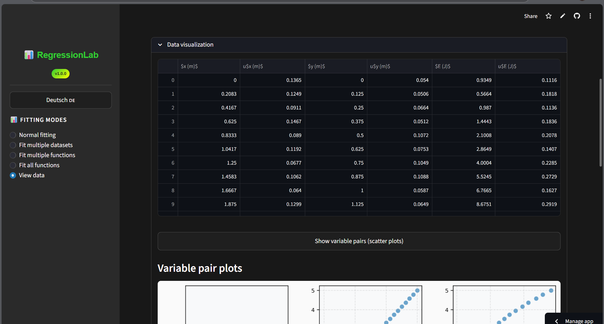
Mode 4: View Data
Purpose: View data from a file without performing any fitting. Includes transform, clean, and download options.
Steps:
Select Mode:
In the sidebar, select “View Data” (or “Mirar datos” in Spanish).
Upload Data:
Click “Browse files” or drag and drop your file.
Supported formats: CSV, XLSX, TXT.
View Data:
Expand the data section to see the table.
Click Show variable pairs (or equivalent in your language) for scatter matrix (pair plots).
If there are more than 10 variables, a multiselect appears to choose which variables to display (max 10 for readability).
Transform Data (optional):
Select a transform from the dropdown: FFT, FFT magnitude, inverse FFT, DCT, inverse DCT, log, log10, exp, sqrt, square, standardize (z-score), normalize [0,1], Hilbert, inverse Hilbert, envelope (Hilbert), Laplace (discrete), inverse Laplace, cepstrum (real), Hadamard (Walsh), inverse Hadamard.
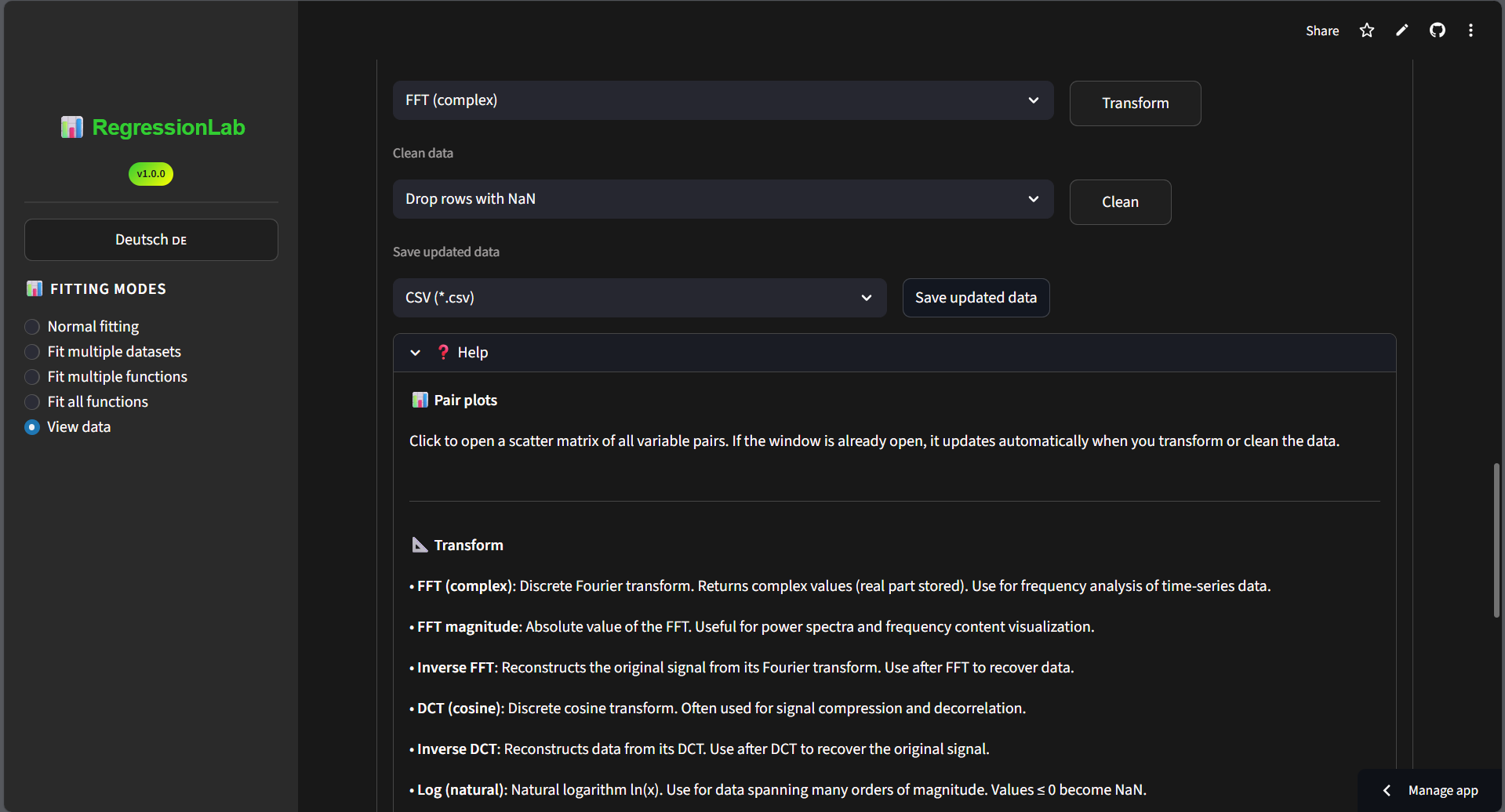
Click Transform to apply. The table updates immediately.
Clean Data (optional):
Select a cleaning option: drop NaN rows, drop duplicates, fill NaN (mean/median/zero), or remove outliers (IQR or z-score).
Click Clean to apply. The table updates immediately.
Download Updated Data (optional):
Choose format (CSV, TXT, XLSX) from the dropdown.
Click the download button to save the current (possibly transformed/cleaned) data.
Help (optional):
Expand the Help section for a reference with pair plots, transform options (each with a detailed description), clean options (each with a detailed description), and save. Content available in Spanish, English, and German.
Use case: Inspect columns, check data quality, transform or clean data, visualize variable pairs, or download processed data before deciding on a fitting mode.
Mode 5: Total Fitting
Purpose: Automatically test ALL available equations on your dataset.
Steps:
Select Mode:
In sidebar, click “Total Fitting”.
Upload Data:
Upload your data file.
Select Variables:
Choose X and Y variables.
Enter plot name.
Plot Options (optional):
Show plot title: Checkbox to show or hide the title on all plots. Default from
PLOT_SHOW_TITLEenv var.
Run Total Fitting:
Info message shows: “Total Fitting: [N] equations”.
Click “Total Fitting” button.
Progress bar shows completion.
All predefined equations fitted automatically.
Takes longer than other modes.
Review All Results:
Comprehensive results for all equation types.
Scroll through to find the best fit.
Look for highest R² value.
Use Cases:
Exploratory data analysis.
No prior knowledge of expected relationship.
Creating comprehensive reports.
Educational purposes (see all function types).
Example Workflow:
1. Upload: mystery_data.csv
2. X: x, Y: y
3. Plot name: "comprehensive_analysis"
4. Click "Total Fitting"
5. Wait for all 13+ equations to fit
6. Scan through results:
   - Linear: R²=0.60
   - Quadratic: R²=0.65
   - Sin with phase: R²=0.99 ← Best!
   - Logarithmic: R²=0.45
   - ... etc.
7. Use "Sin with phase" for this data
Data Upload
Supported Formats
CSV (
.csv): Comma-separated values.Excel (
.xlsx): Microsoft Excel files.TXT (
.txt): Tab-separated or space-separated text files.
File Size Limits
Online version: Limited by Streamlit Cloud (typically 200 MB).
Local version: Limited by your computer’s memory.
Upload Methods
Click “Browse files”: Opens file picker dialog.
Drag and drop: Drag files from your file manager into the upload area.
Multiple File Upload
Hold Ctrl (Windows/Linux) or Cmd (Mac) while selecting.
Or drag multiple files at once.
Only available in “Multiple Datasets” mode.
Data Preview
After upload, expand “Show Data” to see:
First and last rows.
All columns.
Data types.
Verify data loaded correctly.
Understanding Results
Results are shown in three columns, then the plot, then the download button.
Column 1: Equation
Formula (if available): The generic equation form (e.g. y = mx + n).
Formatted equation: The equation with fitted parameter values (e.g. y = 5.123·x + 2.456).
Uses standard mathematical symbols (·, ², etc.).
Column 2: Parameters
Fit parameters (e.g. a, b, c or m, n) with uncertainties and confidence intervals:
Each parameter: value and uncertainty (e.g. m = 5.123 , σ(m) = 0.045).
IC 95%: 95% confidence interval for each parameter.
Column 3: Statistics
R²: Coefficient of determination.
RMSE: Root mean square error.
χ²: Chi-squared.
χ²_red: Reduced chi-squared.
ν (g.l.): Degrees of freedom.
Plot Components
Data Points:
Red circles (or other markers).
Error bars if uncertainties provided.
Your original measurements.
Fitted Curve:
Black line (or configured color).
Smooth curve through data.
Based on fitted equation.
Axis Labels:
X-axis: Your X variable name.
Y-axis: Your Y variable name.
Legend (if shown):
Equation with parameters.
R² value.
R² Value (Coefficient of Determination)
Interpretation:
R² = 1.0: Perfect fit (rare in real data).
R² > 0.95: Excellent fit ✓.
R² > 0.85: Good fit ✓.
R² > 0.70: Acceptable fit ⚠️.
R² < 0.70: Poor fit - try different equation ✗.
What it means:
Percentage of variance explained by the model.
R² = 0.95 means 95% of variance explained.
Higher is better.
Downloading Plots
Scroll to the result you want (plot is above the download button).
Click the “📥 Download” button below the plot.
File is saved with the configured format (default PNG); filename:
[plot_name].png(or.pdfif configured).
Download Tips:
Download all plots you need before closing the browser.
Plots are high-resolution (configured DPI).
If the app is configured for PDF output, the in-app preview is shown as PNG but the downloaded file is PDF.
Tips and Best Practices
Performance Tips
Use local version for large datasets: Faster than online.
Close unused browser tabs: Frees memory.
One mode at a time: Don’t switch modes mid-analysis.
Clear results: Refresh page to clear old results and free memory.
Data Tips
Check data preview: Always expand “Show Data” to verify upload.
Name columns clearly: Use descriptive names like “time_s”, “voltage_V”.
Remove headers in Excel: Only column names in first row, data starts row 2.
Consistent units: Ensure all data uses the same units.
Workflow Tips
Start with Normal Fitting: Test single equation first.
Use Checker for exploration: When uncertain about best equation.
Use Total for comprehensive analysis: When time permits.
Document your results: Download all relevant plots.
Uncertainty Handling
If your data has uncertainties:
Name columns
ux,uy(lowercase ‘u’ + variable name).Example: for variable
time, uncertainty column isutime.Error bars appear automatically in plots.
Fitting is weighted by uncertainties.
Custom Formula Tips
Test simple formulas first: Try
a*xbefore complex expressions.Use parentheses:
a/(1+b*x)nota/1+b*x.Available functions:
np.sin(),np.cos(),np.exp(),np.log(),np.sqrt().Check parameter count: Must match number of parameters defined.
Troubleshooting
Upload Issues
Problem: File won’t upload.
Solutions:
Check file format (CSV, XLSX, TXT only).
Try smaller file.
Check internet connection (online version).
Refresh page and try again.
Fitting Fails
Problem: “Fitting error” message appears.
Possible causes:
Not enough data points (need at least 5-10).
Data doesn’t match equation type.
Infinite or NaN values in data.
All Y values are the same.
Solutions:
Check data for errors.
Try different equation type.
Ensure sufficient data points.
Remove outliers or bad data.
Results Not Showing
Problem: Clicked fit button but no results appear.
Solutions:
Wait for processing (check for spinner).
Scroll down (results may be below viewport).
Check browser console for errors (F12).
Refresh page and try again.
App is Slow
Problem: App responds slowly or freezes.
Solutions:
Use local version instead of online.
Reduce dataset size.
Close other browser tabs.
Clear browser cache.
Refresh the app.
Download Doesn’t Work
Problem: Can’t download plots.
Solutions:
Check browser’s download settings.
Allow downloads from streamlit.app domain.
Try right-click → “Save image as”.
Use different browser.
Keyboard Shortcuts
While Streamlit doesn’t have extensive keyboard shortcuts, these work:
Ctrl+R / Cmd+R: Refresh the app.
F5: Refresh the page.
F11: Full screen mode.
Ctrl+Plus / Cmd+Plus: Zoom in.
Ctrl+Minus / Cmd+Minus: Zoom out.
Mobile and Tablet Usage
The Streamlit interface is responsive and works on mobile devices:
Recommendations:
Use landscape orientation for better plot viewing.
Tap and pinch to zoom plots.
Use tablet or larger for easier interaction.
Desktop recommended for serious work.
Advanced Features
Session Persistence
Results persist during your browser session.
Refresh clears all results.
Online version: sessions timeout after inactivity.
Multiple Tabs
You can open multiple browser tabs with RegressionLab:
Each tab is independent.
Useful for comparing different analyses.
Be mindful of memory usage.
Appearance and theme
The Streamlit UI uses the same configuration as the Tkinter app. Colors and fonts come from .env (or the Tkinter Configure dialog):
Background and text:
UI_BACKGROUND,UI_FOREGROUNDSidebar: Slightly lighter than the main area for separation
Buttons and accents:
UI_BUTTON_BG,UI_BUTTON_FG, etc.Fonts:
UI_FONT_FAMILY,UI_FONT_SIZE
So changing the theme in .env (or in Tkinter’s configuration) affects both the desktop and the web interface consistently.
Differences from Tkinter Version
Streamlit has:
✓ Modern, web-based interface.
✓ Same theme and configuration source (
.env/ config): colors, fonts, and layout rules match the Tkinter app where applicable (sidebar slightly lighter than main).✓ Easy sharing via URL.
✓ Mobile/tablet support.
✓ No installation needed (online).
✓ Loop-like workflow: in Normal Fitting you can enable “loop fitting” and then fit another file with the same equation without changing mode; in Multiple Datasets you can upload another set of files and run again.
Streamlit differs:
File input is by upload only (no local file browser).
No configuration panel in the sidebar (language and mode only); change settings in
.envor via Tkinter’s Configure menu.Results layout: three columns (Equation, Parameters, Statistics), plot, then download button.
If output format is PDF, the in-app preview is PNG and the download is PDF.
Prediction window and multidimensional fitting (custom formulas with 2+ variables, 3D/residuals plots) are currently available in the Tkinter (desktop) version.
View Data mode in Streamlit has the same transform, clean, and download options as Tkinter.
When to use each:
Streamlit: Quick analysis, sharing, accessibility.
Tkinter: Offline, local file browsing, in-app configuration dialog, extra features.
Next Steps
Learn Tkinter: See Tkinter Guide for desktop version.
Customize: Configure appearance in Configuration Guide.
Extend: Learn to add functions in Extending RegressionLab.
Happy fitting! If you encounter issues, check the Troubleshooting Guide.